Diagnostics for GLMs

Home

How does one find outliers, influential observations?

How about prediction intervals, confidence intervals?

https://www.sagepub.com/sites/default/files/upm-binaries/21121_Chapter_15.pdf [Textbook]

Leverage Score Estimation

https://icml.cc/2012/papers/80.pdf [2012 Fast approximation of matrix coherence and statistical leverage]

Firstly, we have to derive the hat matrix for GLMs. We find that:

Also notice the sum of the leverage scores is equal to the number of parameters in the model.

[BE CAREFUL NOT ALWAYS!!! Ie like in Ridge Regression]

However be careful! The TRUE hat matrix is NOT the formula above, but rather:

Ive confirmed the norm between them is off by around p - rank(H).

However, since we only want the leverage scores, we use the trace property cycling property.

However, on further notice, we notice via the Cholesky Decomposition that:

All in all, this optimized routine computes both the variances(beta) and leverage(X) optimally in around:

np^2 + 1/3p^3 + 1/2p^3 + p^2 + np^2 + np + n FLOPS.

Or around:

(2/3)p^3 + (2n)p^2 + (n+1)p FLOPS.

And peak memory consumption:

n/Bp + p^2 + n + p SPACE.

Where B is the batch size.

Now going about estimating the leverage scores or the diagonal hat matrix is a pain. One clearly will be crazy on computing

the full hat matrix then only extracting the diagonals.

Instead sketching comes to the rescue again!

Also notice the maximum leverage score must be 1 [leverage scores are between 0 and 1.]

Also, notice the scaling of the normal distribution sketch.

Now the sketching matrices can be the count sketch matrix.

S2 should NOT be a count sketch matrix, since during the triangular solve.

Notice the error rate. That means in general if the sketching size requires too many observations,

you would rather use the original matrix.

Standardized, Studentized Residuals

Pearson residuals are the per observation component of the Pearson goodness of fit test ie:

Where we have for the exponential family:

Name	Distribution	Range
Poisson
Quasi Poisson
Gamma
Bernoulli
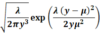
Inverse Gaussian
Negative Binomial

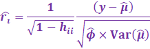
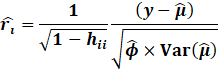
Standardized Pearson Residuals then correct for the leverage scores:

[These are also called internally studentized residuals]

For practical models:

Name	Range
Poisson
Quasi Poisson
Linear
Log Linear
ReLU Linear
CLogLog Logistic
Logistic

The PRESS residuals showcase the difference in the prediction and true value if we

excluded the observation from the model.

These can be proved by using the Sherman Morrison Inverse Identity formula.

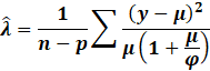
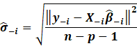
However, in outlier analysis, one generally considers the externally studentized residuals,

which essentially is when the variance is estimated whenever each observation is deleted it.

Minus 1 because one datapoint is deleted each time.

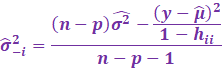
Now to simplify this, we utilize the PRESS residuals:

[ Gray part skips steps which are a bit tedious to showcase 😊 ]

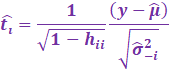
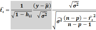
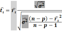
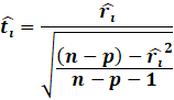
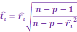
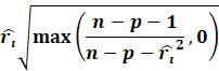
Then the externally studentized residuals utilises this new excluded variance:

However in GLMs, we cannot resort to this estimate for the OLS model.

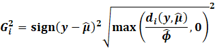
Rather, we first remember the Deviance Residuals:

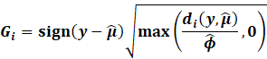
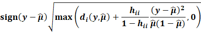
The standardized deviance residuals are then:

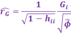
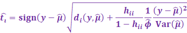
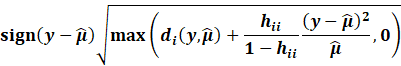
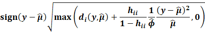
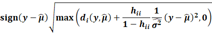
Then, we get the Williams approximation to externally studentized residuals:

Which we find that:

For practical models:

Name
Poisson
Quasi Poisson
Linear
Log Linear
ReLU Linear
CLogLog Logistic
Logistic

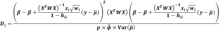
Cooks Distance, DFFITS

Popular methods to detect influential or possible outliers include the Cooks Distance and DFFITS.

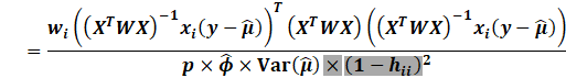
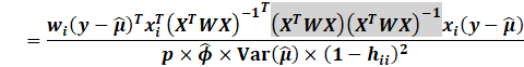
The Cooks Distance is essentially the total change in MSE if an observation is removed.

It shows how much error can be seen in standard deviation units on how the error changes

if an observation is removed.

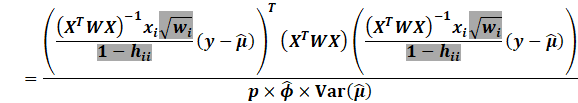
First notice by using the Sherman Morrison inverse formula that:

We then expand:

Generally, a cutoff of 4/n is reasonable. Likewise, one can use the 50% percentile of the F distribution.

Though for large n, this will converge to 1.

On the other hand, DFFITS is a similar measure to the Cooks Distance.

DFFITS rather uses the externally studentized residual, which is more preferred than the Cooks Distance.

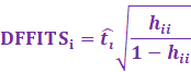
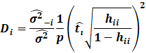
In fact, DFFITS is closely related to the Cooks Distance:

The cutoff value for DFFITS is:

Finally to plot and showcase the possible outliers, one can use for both axes:

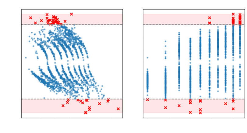
However in practice, the identification of outliers is more complicated than using DFFITS, since DFFITS can suggest

too many outlier candidates. Rather we use the Studentized Residuals vs Leverage plot:

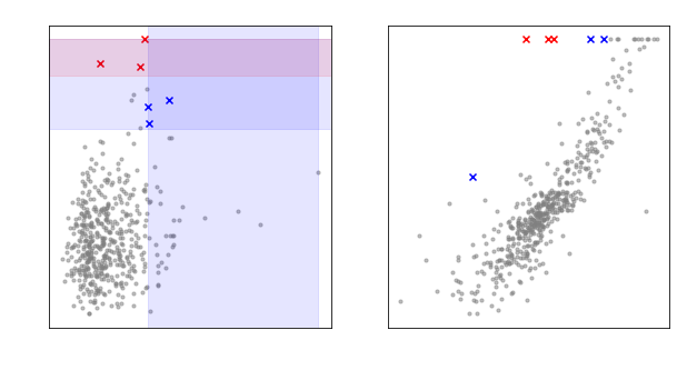
The cutoff is 3 * the studentized residual (ie the residual is 3 standard deviations away from the mean).

Likewise the leverage much be at least 2 times the average leverage.

However, we need to also capture wildly off-putting results. So, we also include anything above 5 standard deviations.

Confidence, Prediction Intervals

Confidence and Prediction Intervals for both new data and old data are super important aspects.

The trick is one utilises the leverage scores.

Remember that:

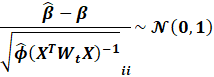
This essentially means that:

Notice how this is NOT the leverage score!!!!!!

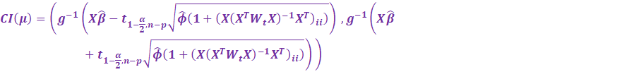
And then for GLMs, via the inverse link function (the activation function):

Then, we have the upper (97.5%) and lower (2.5%) confidence intervals:

Be careful! Its the upper (97.5%) and lower (2.5%) confidence intervals! Not 95%.

For new data points though, we have to estimate the factor. We can do this via:

[Where A is the new data matrix, psi is the new predicted value and z is the new weight]

Remember though previously we performed the Cholesky Decomposition on the variance matrix.

So, we can speed things up by noticing:

[Notice we exclude the new weights]

For Prediction Intervals, we shall not prove why, but there is in fact a +1 factor inside the leverage square root:

Notice if the dispersion parameter is 1 (Poisson, Bernoulli models), then the normal distribution is

used instead of the Student T distribution for the critical values.

License: All content on this page is for educational and personal purposes only.

Usage of material, concepts, equations, methods, and all intellectual property on any page in this publication

is forbidden for any commercial purpose, be it promotional or revenue generating. I also claim no liability

from any damages caused by my material. Knowledge and methods summarized from various sources like

papers, YouTube videos and other mediums are protected under the original publishers licensing arrangements.

Home