Statistical Inference for GLMs

After carefully fitting the coefficients for a GLM, one then must test the significance of them.

We can easily test them via statistical tests.

https://www.sagepub.com/sites/default/files/upm-binaries/21121_Chapter_15.pdf [Textbook]

https://docs.scipy.org/doc/scipy/reference/generated/scipy.sparse.linalg.lgmres.html#scipy.sparse.linalg.lgmres [LGMRES]

Dispersion Parameter Estimation

Recall that:

This means that the final variance of the parameters is:

[Notice W is not weights, but rather the original variance, since we do not cancel the dispersion out]

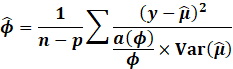
However, we do not know the dispersion parameters. So, we estimate them via the method of moments:

Now lets derive the variance for the generic exponential families:

Name	Distribution	Range
Poisson
Gaussian
Gamma
Bernoulli
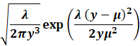
Inverse Gaussian
Negative Binomial

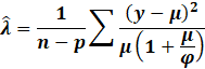
Notice for the Poisson model, to counteract over or under dispersion, we generally let the dispersion parameter to be:

This is called the Quasi Poisson Model

Coefficient Significance

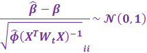
A Wald Test can be used to determine the significance of coefficients, assuming CLT:

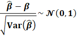
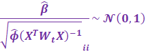
To test the hypothesis that the coefficients are zero,

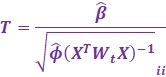
Given a 0.05% significance level, we then perform a two sided Z test:

s = 2 * (1 - scipy.stats.norm.cdf(abs(T)))

However, for when a dispersion parameter is estimated, one must use a 2 sided T test.

s = 2 * (1 - scipy.stats.t.cdf(abs(T), df = n - p))

Likewise for confidence intervals at the 0.05 significance level, we show both Z and T tests.

k = scipy.stats.norm.ppf(1 - 0.05/2)

k = scipy.stats.t.ppf(1 - 0.05/2, df = n - p)

Then, we have the upper (97.5%) and lower (2.5%) confidence intervals:

Be careful! It’s the upper (97.5%) and lower (2.5%) confidence intervals! Not 95%.

In general, if the sample size is large enough, the T distribution converges to a Normal distribution.

At the 0.05 significance level, we have that

However, with the T distribution on less than 10,000 samples, the value is much larger ie:

So, one should keep a table of precomputed values less than 10,000 or so samples,

then clip the value to 1.96.

So finally, we have the following

Name	Distribution	Range	Test Statistic
Poisson
Quasi Poisson
Gaussian
Gamma
Bernoulli
Inverse Gaussian
Negative Binomial

However, for the Quasi Poisson Model, one uses a T distribution.

Degrees of Freedom Estimation

In general inference of many parameters, n-p is taken to be the degree of freedom.

However, in statsmodels and many other statistical packages, rather the actual rank of the matrix is used.

However, when Cholesky or even the modified Cholesky (Levenberg–Marquardt) algorithm is used, one does not

attain the singular values.

Pivoted Cholesky can be used to attain an approximate rank. Likewise, entries which are negative or zero

in the factorization can be considered as rank deficient columns.

Variance Estimation

If the data matrix is exceptionally large, one cannot afford to invert the matrix.

So, we have to find an approximate inverse to the matrix.

The most basic approximation is to just use the diagonal of the weights matrix ie:

However, the error especially for p-value computations is very very bad.

One can also use the Power Method to approximate the top K eigenvalues and eigenvectors, say like 5,

then use these and compute the diagonals ie:

[Notice the clipping of the eigenvalues]

However, the power method find the largest eigenvalues. Since we want the inverse matrix, we rather

want the SMALLEST eigenvalues.

We can do this via the inverse power method.

However, given a large matrix, it becomes infeasible to even solve the system of equations.

One can then use MINRES to solve the system. However, MINRES has bad convergence qualities.

One should rather use LGMRES, which fixes MINRES and converges much faster.

However, this is still prohibitive. Instead sketching comes to the rescue. Assuming weights are positive, we have that:

So the algorithm becomes:

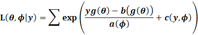
Likelihood and Deviance

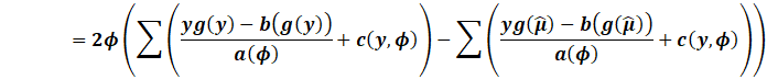
The deviance is the measure of relative importance when comparing 2 models.

The first term is called the saturated model.

This is when we create a new linear model where the predictions are the actual targets themselves!

Notice for the exponential family:

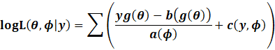
So, for the exponential family:

Name
Poisson
Quasi Poisson
Gaussian
Gamma
Bernoulli
Inverse Gaussian
Negative Binomial

And for practical models:

Name	Range
Poisson
Quasi Poisson
Linear
Log Linear
ReLU Linear
CLogLog Logistic
Logistic

The residual deviance is the difference between this saturated model and the fitted model itself.

For the simple linear regression model we have that:

And for practical models, the case wise deviances:

Name	Range
Poisson
Quasi Poisson
Linear
Log Linear
ReLU Linear
CLogLog Logistic
Logistic

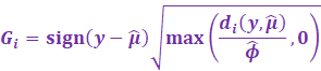
And finally, the deviance residuals are then calculated as:

And the deviance score is calculated as:

AIC, BIC

https://en.wikipedia.org/wiki/Akaike_information_criterion [AIC]

https://en.wikipedia.org/wiki/Bayesian_information_criterion [BIC]

The Akaike Information Criterion determines if a model is a good fit and is not overfit to the data.

It measures the models strengths, and can be used as a way to compare other models.

Choose the LOWEST AIC value.

AIC can be used in the relative likelihood ratio test, where we can compare models.

Say we have 10 models, with the minimum AIC score as MIN.

Then the quantity

Can be used to determine the probability another model can minimise the information criterion.

Say if the minimum was 100, and another model had an AIC of 102.

This means model 2 has a 36.8% chance of minimising AIC rather than the best model.

The strength of a model can be evaluated as follows:

	Comparison
	Hopeless
	Positive
	Strong
	Very strong

The BIC or Bayesian Information Criterion is more advocated since it penalises model complexity.

For extremely large data, high dimensional BIC is rather used, where:

Gamma be can any number greater than 0. Generally set it to zero.

The strength of a model can be evaluated as follows:

	Comparison
	Hopeless
	Positive
	Strong
	Very strong

License: All content on this page is for educational and personal purposes only.

Usage of material, concepts, equations, methods, and all intellectual property on any page in this publication

is forbidden for any commercial purpose, be it promotional or revenue generating. I also claim no liability

from any damages caused by my material. Knowledge and methods summarized from various sources like

papers, YouTube videos and other mediums are protected under the original publishers licensing arrangements.

Home