Linear Regression & Least Squares

Home

How does one estimate the parameters of a linear model?

How about when a matrix is underdetermined or ill conditioned?

How do we determine the best L2 regularization parameter?

Just a refresher for overdetermined systems:

For underdetermined systems:

Recursive Stable Cholesky Decomposition

https://en.wikipedia.org/wiki/Cholesky_decomposition [Wikipedia]

https://en.wikipedia.org/wiki/Denormal_number#Performance_issues [Wikipedia]

https://en.wikipedia.org/wiki/Schur_complement [Wikipedia]

We have already showcased how using Cholesky is paramount to superior speed.

This is because 2 triangular solves (P^2) can be used:

However, actually performing the Cholesky decomposition has many issues.

The first issue is how does one actually compute the upper triangular factor U?

From Wikipedia, the Cholesky Crout algorithm proceeds column wise:

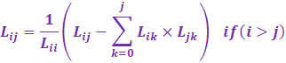
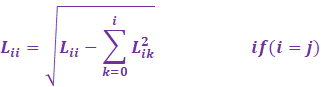
In code:

for (int i = 0; i < n; i++)

{

for (int j = 0; j < i; j++)

{

float s = 0;

for (int k = 0; k < j; k++)

s += A[i, k] * A[j, k];

A[i, j] = (A[i, j] - s) / A[i, i];

}

float s = 0;

for (int k = 0; k < i; k++)

s += A[i, k] * Ai[i, k];

A[i, i] = sqrt(A[i, i] - s);

}

However, we can optimize the code by noticing that our matrix was originally Fortran Contiguous, so each column is

accessed optimally. Likewise, store the divisions and use multiplication instead.

for (int i = 0; i < n; i++)

{

float *__restrict Ai = &A(i, 0);

for (int j = 0; j < i; j++)

{

float *__restrict Aj = &A(j, 0);

float s = 0;

for (int k = 0; k < j; k++)

s += Ai[k] * Aj[k];

Ai[j] = div[j] * (Ai[j] - s);

}

float s = 0;

for (int k = 0; k < i; k++)

s += Ai[k] * Ai[k];

const float aii = sqrt(Ai[i] - s);

Ai[i] = aii;

div[i] = 1/aii;

}

The issue is that the above has many issues, namely the highlighted.

The first issue is that the square root can become negative. These also indicate rank deficient columns.

We counteract this by adding a check. We also notice that using FLT_MAX is SLOW due to underflow and denormals.

(Wikipedia says it can be 100 times slower). And finally, we have to set all rank deficient columns to zero.

So, we rather use 1/EPS which is around 8.3e+6 compared to FLT_MAX which is 3.4e+38.

Likewise, we set all elements smaller than EPS to 0.

for (int i = 0; i < n; i++)

{

float *__restrict Ai = &A(i, 0);

for (int j = 0; j < i; j++)

{

float *__restrict Aj = &A(j, 0);

float s = 0;

for (int k = 0; k < j; k++)

s += Ai[k] * Aj[k];

Ai[j] = div[j] * (Ai[j] - s);

}

float s = 0;

for (int k = 0; k < i; k++)

s += Ai[k] * Ai[k];

const float aii = (Ai[i] - s);

Ai[i] = (aii <= sqrt(EPS)) ? (1/EPS) : sqrt(aii);

div[i] = (aii <= sqrt(EPS)) ? (0) : (1/sqrt(aii));

}

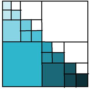
However, the routine above is exceptionally slow for large matrices. We rather have to use divide and conquer

to recursively split the matrix into halves, then use STRSM and SSYRK to perform a Schur Complement.

We first perform Cholesky on the top left corner.

Then, we solve with STRSM then use SSYRK.

We then have the transformed matrix:

We then perform Cholesky on the bottom right corner.

We can do this recursively. The main benefit is in the old routine, Cholesky / STRSM / SSYRK takes P^3 time.

Well Cholesky 1/3P^3 FLOPS, STRSM and SSYRK both 1/2P^3 FLOPS.

If we do a simple calculation of depth = 3, we will find the following FLOPS:

This means the summation becomes:

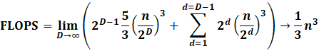
However notice how the original Cholesky takes 1/3n^3 FLOPS. So what’s the big deal?

Parallelization! STRSM and SSYRK are extremely easy to parallelize. In fact with K cores, assume a 1/K improvement.

Cholesky is much harder to parallelize, since there are synchronization steps at each row. Assume a 1/log2(K) improvement.

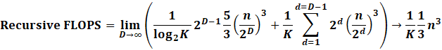
Now we see the benefit! An approx sqrt(K) improvement. Ie if you had 16 cores, expect a 4 times improvement.

Jacobi Preconditioning & Standardization

https://www.netlib.org [SPSTRF]

https://www.gnu.org/software/gsl/doc/html/linalg.html#c.gsl_linalg_cholesky_scale [Jacobi Preconditioning]

Also, to reduce the condition number of the matrix, one can use Jacobi Preconditioning.

Another obvious way to counter large condition numbers is to first standardize the matrix.

IF YOU DO STANDARDIZATION TURN OFF JACOBI PRECONDITIONING!

However, we don’t want to compute the standardized data since that’ll take a lot of memory.

We first precompute the reciprocal of the standard deviations, then expand the above equation.

We also reset the reciprocal to 0 if the original standard deviation was 0.

However notice the following relation:

Which then we simplify the above to:

In other words, we do not need to create a new memory space for the standardized X!

We can precompute XTX, then subtract the mean factor, then multiply by the reciprocal standard deviation.

In all, the number of operations reduces from NP FLOPS to now P^2 FLOPS.

Likewise memory usage has reduced from an extra NP space to now virtually 0!!

Be careful of the N factor when you multiply the 2 means!

However, sadly, for large dimensional data, ie p > n, the above method fails.

Since we have:

The above does NOT simplify sadly, so the only way to compute the above is to actually compute

the standardized data. Though if memory is an issue, we can compute column subsets then update XXT.

For matrix matrix multiplication, we have a similar phenomenon:

So, we first copy and scale V by the scale factor. Then perform a simple matrix vector multiply

To obtain the correction factor for each column.

This means we can reduce memory usage from NP to now PK. This method is not

suggested if K > N.

However in practice, especially for solving with Cholesky, one should NOT minus the mean.

The removal of the mean can in fact REDUCE accuracy!!

However for PCA, mean removal is inevitable, or else clusters become incorrect.

So, for both XTX and XXT:

Ridge Regression & LOOCV

http://pages.stat.wisc.edu/~wahba/ftp1/oldie/golub.heath.wahba.pdf [1979 Generalized Cross Validation for Choosing a Good Ridge Parameter]

https://arxiv.org/abs/1803.03635 [2018 The Lottery Ticket Hypothesis]

Ridge regression is particularly useful for reducing the norm of the parameters.

It in fact has a closed form solution:

For underdetermined systems, Cholesky can become rank deficient, and fail. So we have to add regularization. A good heuristic:

This is mostly guaranteed to attain good accuracy. In fact, this was the tolerance factor from LAPACKs pivoted Cholesky (SPSTRF).

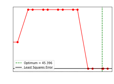
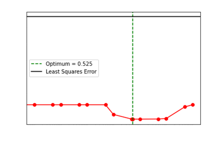
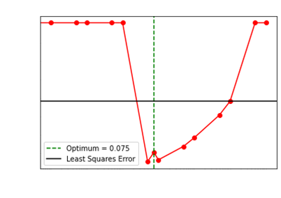
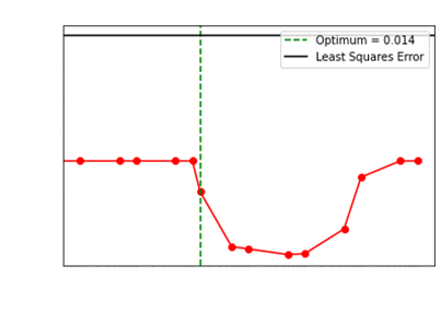
We showcase how our choice of the optimum regularization performs:

Levenberg Marquardt Modified Correction

https://en.wikipedia.org/wiki/Levenberg%E2%80%93Marquardt_algorithm [Wikipedia]

Sadly for very ill conditioned matrices, simply using stable Cholesky above still fails to converge at all.

So we invoke Levenberg Marquardt’s correction (ie the LM algorithm).

Instead of a simple Ridge regularization, we scale according to the diagonal elements.

However this method disregards collinear columns. If 2 columns are perfectly corrected, LM will still fail.

So, we inject some deterministic jitter.

Now, we can set the regularization parameter to a small number ie epsilon * 10. Choosing epsilon

causes the addition to turn to not updating anything.

We then shift the brackets around.

However for extremely ill conditioned matrices, even the LM algorithm fails. So, we use our optimal L2 regularization plus the LM

algorithm to make the final system always converge.

(c) Copyright Protected: Daniel Han-Chen 2020

License: All content on this page is for educational and personal purposes only.

Usage of material, concepts, equations, methods, and all intellectual property on any page in this publication

is forbidden for any commercial purpose, be it promotional or revenue generating. I also claim no liability

from any damages caused by my material. Knowledge and methods summarized from various sources like

papers, YouTube videos and other mediums are protected under the original publishers licensing arrangements.

Home